Introduction to LSTM networks

This post is intended as a brief introduction to recurrent neural networks, focusing on long-short term memory cells, for those with a mathematical background. I highly recommend reading the original and great paper LSTM by Hochreiter and Schmidhuber.

Overview

Artificial neural nets (ANNs or neural nets for short) are special types of functions defined on spaces of sequences. In practice, a neural net transforms sequences \( \left\{ x _ n \right\} \) of points sampled (perhaps with added noise) from some manifold \(M \subseteq \mathbb{R}^{D_{\mathrm{in}}}\) in some “useful” way. Examples of “useful” transformations will often reduce dimension or, if the manifold \(M\) is supposed to be Riemannian, lower the curvature.

More precisely, a length \(\kappa\) input signal is a sequence

of vectors in our input space \(\mathbb{R}^{D_{\mathrm{in}}}\). The length \(\kappa\) is usually not too important for theoretical considerations; we will assume it to be some finite number. Similarly, a length \(\kappa\) output signal is a sequence

We let \(\mathfrak{X}(\kappa)\) and \(\mathfrak{Y}(\kappa)\) denote the spaces of length \(\kappa\) input and output signals respectively. A neural network can then be described as a function \(F_{\mathrm{net}} \colon \mathfrak{X}(\kappa) \rightarrow \mathfrak{Y}(\kappa)\) constructed by networking “simple” functions together in a manner prescribed by some underlying directed graph structure.

Static Structure

A neural network structure is a graph \((V, E)\) where:

• the vertex set \(V = \{\theta_1, \dots, \theta_N\}\) is taken to represent a collection of neurons,
• elements the edge set \(E\) represent synapses between neurons in the network. The synapse connecting a neuron \(\theta_i\) to \(\theta_j\) will be denoted by \(\theta_i \to \theta_j\).

For each neuron we define the two numbers

Neurons can be classified based on whether they accept input, produce output, or neither. Corresponding to this there is a decomposition

where

• \(\texttt{input}\) contains neurons that accept input from the outside world. Since no synapse can terminate at an input neuron, we have the definition

• \(\texttt{hidden}\) contains neurons that neither accept input or produce output. These neurons perform intermediate steps of computation and can be characterized by the definition

• \(\texttt{output}\) contains neurons that send output into the world. No synapses can begin at such neurons, so we make the definition

Notice that we have identities relating the cardinalities of \(\texttt{input}\) and \(\texttt{output}\) to the dimensions \(D_{\mathrm{in}}\) and \(D_{\mathrm{out}}\) of the form

Each non-\(\texttt{input}\) neuron \(\theta_i \in V\) is assigned an activation function \(f_i \colon \mathbb{R} \rightarrow [0, 1]\). The activation function \(f_i\) will govern the individual dynamics of \(\theta_i\). (A typical choice of activation function is the logistic function \(f(x) = \frac{1}{1 + e^{-x}}\)) Similarly, each synapse \(\theta_i \to \theta_j\) is assigned a weight \(w_{ij} \in \mathbb{R}\). These weights serve as parameters used to adjust the dynamics of a neural network in order to obtain some desired behaviour.

Notation: We write \(\theta_i \xrightarrow{w_{ij}} \theta_j\) to denote a synapse together with its weight, \(\sum_{\underline{i}\to j}^{} \) to denote a sum over all synapses originating at \(\theta_i\), and \(\sum_{i \to \underline{j}}^{}\) for a sum over synapses terminating at \(\theta_j\).}

If a network structure does not contain any cyclic connections, it is called a \textit{feed-forward} structure. If there are cycles, we say the structure is \textit{recurrent}. We shall focus on feed-forward networks for, as we shall see later, there exists a procedure for converting recurrent nets into feed-forward ones. We will generally reason about recurrent networks by converting them into feed-forward nets.

Dynamic Structure

Fix some non-\(\texttt{input}\) neuron \(\theta_i \in V\). At each time \(t\), this neuron has a state \(\theta_i(t) \in [0, 1]\). (Alternatively, we could require \(\theta_i(t) \in [-1, 1]\). In this case, activation functions like \(f_i(x) = \tanh(x)\) are used instead.) A state of \(0\) means the neuron is totally inactive, while a state of \(1\) indicates the neuron is fully active. In order to compute the state \(\theta_i(t)\), we need to know the inputs to \(\theta_i\) at time \(t\). Define the sum input \(s_i(t)\) to \(\theta_i\) at time \(t\) by

The state of \(\theta_i\) at time \(t\) is computed from the sum input by composing with the activation function:

Notice that the state at time \(t\) depends on the state of all inputs to \(\theta_i\) at time \(t-1\). Proceeding recursively, we see \(\theta_i(t)\) depends on the the state of number of upstream neurons at various times in the past. If instead \(\theta_i\) is an \(\texttt{input}\) neuron, we simply set \(\theta_i(t) = x^i(t)\). At time \(t_0\) we set all non-input states to \(0\).

Let us now restrict our attention momentarily to feed-forward networks. We can get a sense for how data flows through a feed-forward neural network by considering the derivatives \(\frac{\partial \theta_i(t)}{\partial\theta_j(t - q)}\). These derivatives indicate how much the state \(\theta_i(t)\) depends on the the output of another neuron \(\theta_j\) at time \(t - q\). We can derive a recursive algorithm for computing these partials by applying the chain rule:

Here we take the derivative of \(\theta_i(t)\) with respect to the states of all neurons \(\theta_k\) receiving input from \(\theta_j\) at time \(t - q + 1\). Then we take the derivatives of the \(\theta_k\) with respect to \(\theta_j\). Since this is a direct connection, it is an easy computation:

The derivatives \(\frac{\partial \theta_i(t)}{\partial\theta_k(t-q+1)}\) are then computed recursively. \sidenote{Note that we need the feed-forward hypothesis on \((V, E)\) to ensure this recursion terminates.}

In order to get a more explicit formula than equation (\ref{eq:dataflow}) we need to introduce some new notation. Suppose we have a chain of synapses \begin{equation} \label{eq:pathdefn} \theta_i = \theta_{i_0} \to \theta_{i_1} \to \cdots \to \theta_{i_n} = \theta_j \end{equation} containing no cycles connecting the neuron \(\theta_i\) to \(\theta_j\). We call such a chain a length \(n\) \textit{path} from \(\theta_i\) to \(\theta_j\). Note that we can completely describe the path in (\ref{eq:pathdefn}) by the \(n\)-tuple \((i_0, i_1, \dots, i_n)\). This is the tuple of indices of neurons visited along the path. We write \(\mathcal{P}_{ij}(n)\) for the set of all length \(n\) paths from \(\theta_i\) to \(\theta_j\). With this notation and a simple induction combining equations (\ref{eq:dataflow}) and (\ref{eq:lvl1dataflow}), we arrive at the more explicit formula

Observe that if

for all \(1 \leq m \leq q\) then the largest product in equation (\ref{eq:bigeq}) blows-up rapidly as \(q\) goes to \(\infty\). In this case, we have a “hyper-sensitivity” of \(\theta_i\) on \(\theta_j\) as the depth parameter \(q\) gets large. On the other hand, if

for all \(1 \leq m \leq q\) then the largest product in (\ref{eq:bigeq}) vanishes rapidly as \(q\) tends to infinity. This means, for instance, that deep networks initialized with small initial weight values will have very limited expressivity relative to their depth. As we shall see, these two phenomena have important implications regarding the ability of recurrent networks to handle very long input signals. (Very long here meaning \(\kappa > 1000\), say.)

Training neural networks

As was mentioned before, the weight-set \(w_{ij}\) is used to control the functionality of a given neural network. The process of training neural net amounts to making updates to these weights in order to bring out some desirable behaviour. To make the dependence of a neural net on the weight matrix \(w = (w_{ij})\) explicit, we write \(F_{\mathrm{net}}(w; x(t_k))\). In order to model the idea of “desired” behaviour of a neural net, we define a training signal to be a sequence

The sequence \( \{\tau(t_k)\} \) is intended to represent the target output values of the network given the input signal \(\{x(t_k)\} \). An error function is a smooth function

The value \(E(F_{\mathrm{net}}(w; x(t_k)), \tau(t_k))\) measures the extent to which the network output deviates from the target value at time \(t_k\). A typical choice of error function is the (scaled) squared Euclidean norm \(E(x, y) = \frac{1}{2} \left| x - y \right|^2\). This is the error function we shall use. The total error for the training pair \(\{(x(t_k), \tau(t_k))\}_{k=1}^\kappa\) given the weight matrix \(w\) is the sum

The goal of the training process can then be seen as that of minimizing the total error \(e(w)\).

Descent based training

Let \(w_0\) denote the initial weight matrix of some neural network \(F_{\mathrm{net}}\). The total error is a smooth function of the weights, so we can apply gradient descent to select an updated weight set \(w_1\) such that \(e(w_1) < e(w_0)\). In other words, since the function \(e(w)\) decreases most rapidly in the direction of the negative gradient \(-\nabla e(w_0)\), we can choose

If the learning rate \(\gamma > 0\) is well chosen, we will have \(e(w_1) < e(w_0)\) as desired.

In order to understand this approach to training, let us compute the weight-space error gradient \(\nabla e(w)\). (In particular, we shall be interested in the shortcomings of this approach as applied ``out of the box’’. The LSTM architecture was developed precisely to address these shortcomings.) In fact, since \(e(w)\) is just a linear combination of the functions

for \(k \in \{0, \dots, \kappa\}\), it will be enough to compute the partial derivatives \(\frac{\partial E}{\partial w_{ij}}\). To this end we fix some synapse \(\theta_i \xrightarrow{w_{ij}} \theta_j\), some time \(t \in \{0, \dots, \kappa\}\), and apply the chain rule to obtain

The terms \(\frac{\partial \theta_l(t)}{\partial\theta_j(t-q)}\) were already computed in equation (\ref{eq:bigeq}). This algorithm for computing the error is called backpropagation.

In light of equation (\ref{eq:errorflow}), the remarks following equation (\ref{eq:bigeq}) have important implications for error flow through the network. In this case we see that \(|f_{i_m}’(s_{i_m}(t-m)) w_{i_mi_{m-1}}| > 1\) for all \(1 \leq m \leq q\) then the error blows-up as it is propagated backwards through the network. If \(q\) gets too large, weights receive large and often conflicting error signals leading to rapidly oscillating weights and unstable learning. If instead \(|f_{i_m}’(s_{i_m}(t-m)) w_{i_mi_{m-1}}| < 1\) then the error quickly vanishes as it propagates backward through the network. In this case the weights are updated so slowly that nothing can be learned in an acceptable amount of time.

Unrolling a recurrent network

The procedure used to convert recurrent networks into feed-forward networks is called unrolling. We describe this procedure now in order to apply the above analysis to the recurrent network case.

Let \(F_{\mathrm{net}} \colon \mathfrak{X}(\kappa) \rightarrow \mathfrak{Y}(\kappa)\) be a recurrent neural network with network structure \((V, E)\). We construct a new neural net \(F_{\mathrm{net}}^\ast\) with feed-forward network structure \((V^\ast, E^\ast)\) as follows:

• \(V^\ast\) is the disjoint union of \(\kappa\) copies of \(V\), i.e. \(V^\ast = V_0 \sqcup V_1 \sqcup \cdots \sqcup V_\kappa\). The element of \(V_t\) corresponding to a neuron \(\theta_i \in V\) is denoted \(\theta_i^t\). The activation function of a neuron in \(V^\ast\) is the same as its counterparts in \(V\).

• For each synapse \(\theta_i \to \theta_j \in E\), we have synapses \(\theta_i^t \to \theta_j^{t+1} \in E^\ast\) for each \(t \in \{0, \dots, \kappa -1 \} \). Like before, the weights \(w_{ij}^t\) on the synapses in \(E^\ast\) are the same as their counterparts in \(w_{ij}\in E\).

The neural net \(F_{\mathrm{net}}^\ast\) that arises from \((V^\ast, E^\ast)\) given the construction above is feed-forward and so can be trained using the backpropagation algorithm. Notice that at the end of training, the weights \(w_{ij}^t\) might vary with \(t\). To compensate for this, the updated weight set applied to \(F_{\mathrm{net}}\) at the end of training is the average of the \(w_{ij}^t\). In other words, the weights applied to \(F_{\mathrm{net}}\) after training are \(w^{\mathrm{avg}}_{ij}\) where

As the length \(\kappa\) of the input signals tends to \(\infty\), the depth of the unrolled network \(F _ {\mathrm{net}}^\ast\) also increases to \(\infty\). Now, a length \(n\) path

containing no cycles in the network \(F_{\mathrm{net}}\) will be mapped to paths of the form

in \(F_{\mathrm{net}}^\ast\). In other words, if the length \(n\) path \((i_0, \dots, i_n)\) in \(E\) contains no cycles, its images in \(E^\ast\) are all of length \(n\). However, if a neuron \(\theta_i\) has a self-connection, there will be a length \(\kappa\) path

in the expanded edge set \(E^\ast\). Invoking the analysis following equations (\ref{eq:bigeq}) and (\ref{eq:errorflow}), we see that if the activation functions and/or weights are not well-chosen, there could be serious training implications for recurrent networks in the presence of long input signals. We make this more precise in the next section.

Constant error flow

Suppose we have a recurrent neural network \(F_{\mathrm{net}}\) containing a single self-connected neuron \(\theta_i\). As above, this implies there is a length \(\kappa\) path \((i, i, \cdots, i) \in E^\ast\). Following the computations in (\ref{eq:bigeq}) and (\ref{eq:errorflow}), we see that this path contributes a term

to the value of the derivative \(\frac{\partial\theta_i(t)}{\partial\theta_i(t-\kappa)}\). If

for all \(m\) then this blows up like \(\alpha^\kappa\) (resp. decays like \(\alpha^\kappa\)) as \(\kappa \to \infty\).

In order to avoid exploding or vanishing error, it is necessary to ensure that

There are many conditions we could impose on \(f_i\) and \(s_i\) to guarantee this. Perhaps the simplest way to guarantee (\ref{eq:cec}) holds is to

• require \(f_i\) to be the identity function, that is \(f_i(x) = x\) for all \(x\);
• require the activation of \(\theta_i\) be constant, that is \(\theta_i(t +1) = \theta_i(t)\) for \(0 \leq t < \kappa\).

A singly connected neuron satisfying the above requirements is called a constant error carousel (CEC for short). The condition that \(f_i(x) = x/w_{ii}\) comes from integrating the differential equation (\ref{eq:cec}). The choice \(w_{ii} = 1\) is of course most convenient. Substituting \(x = s_i(t)\) we have

which produces the second condition.

Unfortunately, constant error carousel-type neurons are still too simple to be of much use in applications. When we place the neuron \(\theta_i\) into a larger network, two types of problem arise:

• To keep matters simple, suppose we have a two neuron network with neurons \(\{\theta_1, \theta_2\} \) and synapses \(\{\theta_1 \to \theta_2, \theta_2 \to \theta_2\} \). At times \(t\) where \(\theta_i(t) \neq 0\) we view \(\theta_i\) as storing, or “remembering” some piece of information. At a fixed time \(t\), the weight \(w_{12}\) might either receive an error signal attempting to protect the data currently stored in \(\theta_2\) from the current input from \(\theta_1\), or attempting to allow the input from \(\theta_1\) to flow into \(\theta_2\). Over time this will lead to conflicting learning signals and hence unstable learning.

• Now suppose we have another two neuron network \(\{\theta_1, \theta_2\}\) with synapses \(\{\theta_1 \to \theta_1, \theta_1\to \theta_2\}\). Assume that, at some time \(t\), the CEC neuron \(\theta_1\) is storing a value. Like before, the weight \(w_{12}\) is responsible for learning two tasks, and so will receive conflicting update signals. These update signals will attempt to teach \(w_{12}\) when to emit the information stored in the neuron \(\theta_1\), as well as when to protect the neuron \(\theta_2\) from the contents of \(\theta_1\). As before, these conflicting learning signals lead to unstable learning and rapidly oscillating weights.

In order to address these problems, we introduce the Long Short-Term Memory (LSTM) architecture in the next section.

Long Short-Term Memory

To overcome the problem of conflicting weights, we replace CEC neurons with more complicated LSTM memory cells. A memory cell is a multi-neuron complex centred around a CEC neuron. This complex comes equipped with mechanisms for guarding which information flows into and out of the CEC at a given time \(t\). A multiplicative input gate protects whatever content is being stored in the central CEC neuron from being disturbed by new inputs. Similarly, a multiplicative output gate protects neighbouring neurons from being disturbed by the information stored in the CEC neuron at irrelevant times.

In light of the above, we see that a LSTM cell is a small neural network in its own right. The internal structure of such a cell can be visualized as follows:

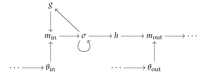
The three neurons on the left form the input gate, \(\sigma\) is called the internal state neuron, and the three neurons on the right form the output gate. The neurons \(g\) and \(h\) are very simplistic, and only receive input from \(\sigma\); \(m_{\mathrm{in}}\) and \(m_{\mathrm{out}}\) are called multiplicative neurons because they simply multiply their inputs together. When reasoning about memory cells we typically “collapse” the internal structure and choose instead to think of the whole cell as a single neuron.

In order to better understand LSTM cells, we study the individual components in detail. We fix some memory cell \(c_j\) and denote the sum input to \(c_j\) at time \(t\) by \(s_{\mathrm{in}}(t)\).

LSTM input gate

An input gate consists of three neurons which we denote by \(\{g, \theta_{\mathrm{in}}, m_{\mathrm{in}}\} \). For convenience we use the same symbols to refer to the associated activation functions. As above, these neurons are connected in the pattern \(g \rightarrow m_{\mathrm{in}} \leftarrow \theta_{\mathrm{in}}\). The activation functions \(g\) and \(\theta_{\mathrm{in}}\) can be arbitrary smooth functions \(\mathbb{R} \to [0, 1]\), but logistic functions are typical choices for both. Notice that \(m_{\mathrm{in}}\) is the only neuron with a synapse leaving the input gate. This means that the output of \(m_{\mathrm{in}}\) represents the output of the entire input unit. We compute the state \(m_{\mathrm{in}}(t)\) (and hence the state of the entire input gate at time \(t\)) by the formula

This formula can be understood as follows. First, \(\theta_{\mathrm{in}}\) combines all inputs to the memory unit at time \(t\) into a single signal. The neuron \(g\) then uses the previous internal state \(\sigma(t-1)\) to “recommend” to the network how much of the signal \(\theta_{\mathrm{in}}\) should be allowed forward into the new internal state. Finally, \(m_{\mathrm{in}}\) multiplies \(g\)’s output with \(\theta_i\) to actually modulate the input signal. When \(g\) outputs a value close to \(1\), \(m_{\mathrm{in}}\) allows most of the input signal to flow into the internal state. An output of \(0\) has the opposite effect of cancelling the input signal.

Internal state neuron

The internal state neuron is simply a CEC neuron with an extra outgoing connection to \(g\).

LSTM output gate

An output gate consists of three neurons \( \{h, \theta_{\mathrm{out}}, m_{\mathrm{out}}\} \) connected like \(h \rightarrow m_{\mathrm{out}} \leftarrow \theta_{\mathrm{out}}\). Again we use the same symbols for the activation functions. As before \(h\) and \(\theta_{\mathrm{out}}\) can be any smooth functions \(\mathbb{R} \to [0,1]\). The output of the entire gate is computed by the neuron \(m_{\mathrm{out}}\) according to the formula

The neuron \(h\) squashes the state value \(\sigma(t)\) into the range \([0, 1]\); \(\theta_{\mathrm{out}}\) recommends how much of this squashed value to release from memory using the net memory unit input \(s_{\mathrm{in}}(t)\). Finally, \(m_{\mathrm{out}}\) implements the recommendation from \(\theta_{\mathrm{out}}\) by multiplying with the value of \(h\).

Conclusion

Recurrent neural networks implementing LSTM neurons have been shown to outperform any other recurrent network architecture in a wide variety of practical applications. Indeed, on tasks like non-segmented handwriting recognition and real-time language translation, LSTM networks often outperform all other machine learning techniques. This is because these tasks require algorithms that can bridge long time delays in their input signals, something LSTM was designed specifically to accomplish. Recent developments include the addition of “forget gates” that allow the memory units to reset themselves spontaneously as the network runs, and mechanisms for allowing LSTM networks to shift attention to subspaces of the input space.