Examples of Neural Adaptation

In this note we investigate how the firing rate response of certain neurons adapts to a constant input stimulus. In particular, we look at the neural adaptivity of frog mechanoreceptors and neocortical pyramidal neurons in rats.

Example 1: Frog Mechanoreceptors

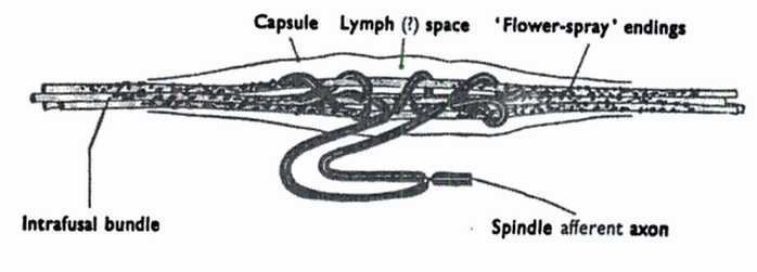
Skeletal muscles in frogs contain “muscle-spindles”, which are sensory nerve fibres wrapped in modified muscle tissue. In the example spindle pictured below¹ we see where the sensory nerve fibres meet with the muscle fibres. Spindles of this form allow the frog to detect when its muscles are stretched in the axial direction.

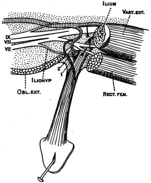
Using a procedure designed by Keith Lucas, it is easy to isolate and manipulate a frog’s sterno-cutaneous muscle. The sterno-cutaneous is a small muscle that attaches to the frog’s sternum on one end and to its skin on the other. In most frogs this muscle contains three or four muscle-spindles. A muscle that has been isolated using Lucas’ procedure is pictured below.²

Using this setup, Adrian and Zotterman were able to record how sterno-cutaneous sensory neurons respond to various types of stretching. They obtained the electrograph below by hanging a 1 gram weight from the muscle and recording the response generated in a single afferent nerve fibre.³

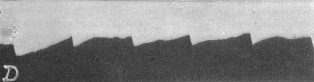
So it would appear that hanging a fixed weight produces a regular firing response in our stretch-sensing neuron. Further experiments with different weights confirm this fact. It turns out that, once a certain threshold is passed, different weights trigger different firing frequencies. As can be seen in the electrograph below, gradually increasing the amount of weight on the muscle results in an increased firing frequency. This is a fairly standard example of rate coding, whereby a neuron encodes information in its firing rate.

All of the experiments we have considered so far look at the response profile in the first few seconds after the weight is hung. If we leave the weight hanging for a long time, the response we observed initially will gradually change until it seems to settle into a regular pattern. Plotting firing frequency against time for muscles stretched by 0.5 and 3 gram weights reveals a power-law type dependency:⁴

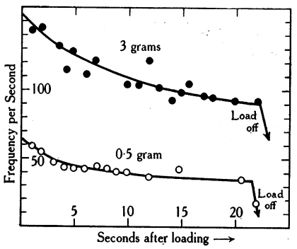
This power-law change in firing response is our first example of neural adaptation.

Example 2: Rat Neocortical Pyramidal Neurons

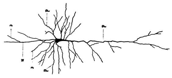
Next we look at experiments carried out by Lundstrom, Higgs, Spain & Fairhall on adaptivity in rat neocortical pyramidal neurons. These are some of the largest neurons in a rat’s brain and are mainly implicated in cognition. Below is a sketch of a human pyramidal neuron⁵, which looks similar to the rat’s.

The neocortex is a thin layer of the brain. Horizontally its neurons are arranged into six layers, usually labed I through VI. As we see in the following diagram⁶, pyramidal neurons are found in the middle layers of the neocortex.

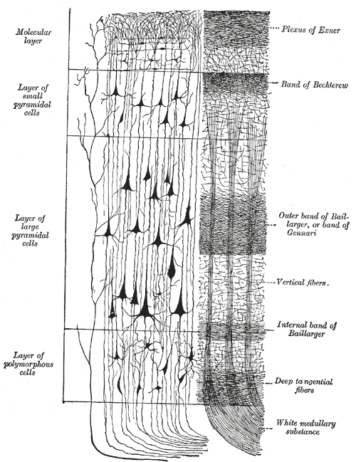
Pyramidal cells in layers II and III project their axons further into the neocortex, while those in deeper layers often have axons that project out of the cortex to areas like the brainstem and spinal cord. Neurons in layer IV receive most of the external connections and project locally to other layers of the neocortex. Vertically the neocortex is arranged into so-called cortical columns. These columns are sometimes thought of as the generic building blocks of the neocortex.

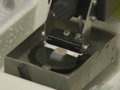
By preparing very thin slices of a rat’s brain (see below⁷), it is possible to isolate neurons in specific layers of the neocortex.

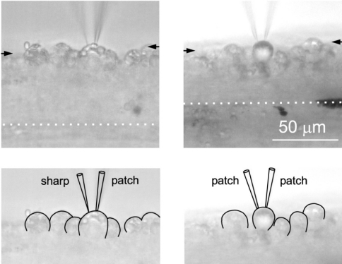
In their experiments, Lundstrom et al used a mixture of whole-cell patch (n = 6) and sharp electrodes (n = 49). These electrodes can be used both to inject a current into a neuron, and to record the resulting electrical response. Examples of both electrode types:⁸

Using this setup, two types of stimulus were used to drive layer II and III pyramidal neurons in the rat neocortex. The first was a simple square wave current (see a. below⁹), and the second was a Gaussian noise current whose standard deviation alternated periodically between two values (see b. below).

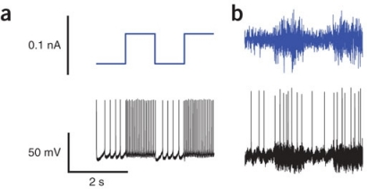
Both stimuli are periodic, say of period \(T\). We are studying responses to constant stimuli, so each period naturally breaks down into two intervals of interest. The first is between time \(0\) and time \(T/2\) when the neuron receives the constant low-current stimulus; the second is from time \(T/2\) to \(T\) when it receives high-current stimulus.

Lundstrom et al experimented with values of \(T\) ranging from \(T = 1 ~\mathrm{sec}\) all the way to \(T = 32 ~\mathrm{sec}\). The averaged firing response rates from these experiments are summarized below. Graphs a and b cover times \([0, T/2]\), while c and d cover \([T/2, T]\). Subject to a bit of normalization, the response profiles are essentially the same for all period lengths \(T\).

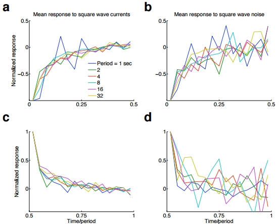
Notice the power-law relationship, just as in the case of the frog mechanorecptor. Note also that:

• Firing frequency trended upwards when given a constant stimulus regime occuring after a high-to-low transition.
• Firing frequency trended downwards when given a constant stimulus regime occuring after a low-to-high transition.